
Project Resonant · paper 02, interactive
Does the physics do the work?
An untrained network of 1,024 coupled oscillators, a linear readout, and spoken digits. How the second paper tests what the oscillators actually contribute, with every model it compares running live in your browser on real recordings.
Twenty held-out clips from AudioMNIST · every model the paper compares · ~25 min read
01 · the questionWhat does the physics add?
In How a machine hears a number I walked from a pressure wave to a network of coupled oscillators that could tell “three” from “eight”. The oscillators were never trained. Their coupling was drawn at random once and never updated, and only a linear readout on top was fitted, and it still read spoken digits at 96%.
That number invites an obvious question, and the first post ended on it: how much of it comes from the oscillators? A good accuracy can come from at least three places that have nothing to do with synchronization physics. The input may already carry most of the answer. The readout may be wide enough to find the answer in almost anything. Or the dynamics may genuinely help. The first guide’s own fine print showed that the readout alone was worth a lot: squeeze its features through a narrow projection and 96.2% fell to 67.3%.
The second paper in this research programme, Spoken-Digit Recognition Without Training, is built to separate those three explanations. It takes a small untrained oscillator network, reads it the same way it reads every alternative, and compares it with models that each remove one ingredient: the dynamics entirely, the oscillation, the coupling. Then it changes the physics one factor at a time, across eight experiments and 6,353 runs.
This page explains that study: what each model is, how they were compared, and why the comparisons are the ones they are, with what the paper found at the end. Every model at the heart of the paper is also running here, in your browser, on real recordings, so you can do the experiment yourself one clip at a time.
02 · oscillatorsOscillators, coupled and uncoupled
An oscillator is anything that cycles: a pendulum, a firefly’s flash, a neuron that fires rhythmically. The simplest mathematical version (Kuramoto) keeps a single number, its phase θ, an angle that advances around a circle. Left alone, it advances at its own natural frequency ω. The interesting part is what happens when many of them can feel each other.
Below are 24 oscillators with different natural frequencies. With the coupling at zero they are an uncoupled population: each turns at its own rate, and their phases smear evenly around the circle. Turn the coupling up and each one starts to be pulled toward the others. Past a threshold, a cluster forms and grows until most of them move together. The white arrow is the order parameter R, the average of all their phases taken as unit vectors: near 0 when they are scattered, near 1 when they are locked.
Written out, each oscillator i in the paper’s network advances by
The network under test
The coupled oscillator network is 1,024 of these: four channels, each a 16 × 16 lattice of 256 oscillators. Row r of every channel is driven by mel band r, lowest at the bottom, so the lattice inherits the ear’s layout. Within a channel, every oscillator acts on every other through a coupling kernel: a 16 × 16 table of weights, one per offset, drawn from N(0, 0.05²). A positive weight pulls a pair toward the same phase, a negative one pushes them apart. The same table applies at every site, which makes the coupling a convolution. Channels do not act on each other: they are four differently drawn copies read side by side, the way a convolutional layer’s channels are.
One more constant bounds the whole thing. A random kernel can amplify some spatial patterns of phase much more than others; the coupling ceiling rescales each channel’s kernel so that its largest amplification is 1. Random kernels here peak between 1.4 and 2.9, so the ceiling always applies, and it sets every channel’s overall coupling strength.
That is the entire model: 1,024 natural frequencies and 1,024 kernel weights, 2,048 numbers, all drawn once from a seed and never updated. The uncoupled oscillator network is the same network with every kernel weight set to zero. Each oscillator keeps its natural frequency, its restoring pull and its input, and none acts on another, so any difference between the two is what the coupling contributes.
03 · the control with memoryLeaky integrators: memory without oscillation
An oscillator network driven by sound is, among other things, a bank of filters with memory. Each oscillator’s state at any moment depends on what it heard recently, weighted toward the recent past. So is a much simpler object, and if the oscillators cannot beat it, their accuracy comes from being filters with memory, not from being oscillators.
That simpler object is the leaky integrator. It holds one number and, every frame, moves a fixed fraction of the way toward its input:
The leaky-integrator bank is 1,024 of these, routed exactly like the oscillator network: band r drives every unit in row r of every channel. Its time constants run on one log-spaced schedule from one frame (16 ms) to one clip (1 s), laid out so that every band is read at every time scale, and its input weights gin are drawn from N(1, 0.1²), the distribution the network draws its natural frequencies from. Nothing about the schedule was tuned: it is a falsification control, not a claim that this is a good design.
It comes in two sizes, because the two models expose different numbers of signals. The state-matched bank has the network’s 1,024 states and 2,048 parameters, but each unit exposes one signal where an oscillator exposes two (sin θ and cos θ). The width-matched bank has 2,048 units, matching the 2,048 signals, at twice the parameters.
04 · the front endSixteen numbers every 16 milliseconds
Every model starts from the same fixed front end, which turns one second of 16 kHz audio into 61 frames of 16 numbers. The first post builds it up piece by piece; here it is with the constants the paper fixed, and why.
| constant | value | why |
|---|---|---|
| sample rate | 16 kHz | Speech carries little above 8 kHz; one second is 16,000 samples. |
| window, hop | 512, 256 samples | A 32 ms window hopping 16 ms: 62.5 frames a second, 61 per clip. No centre padding, so the frame count is exact. |
| mel bands | 16 | One per lattice row, so band r can drive row r directly. |
| log | log(energy + 10⁻⁵) | Loudness is heard on a log scale; the offset keeps silence finite. |
| rescale | (x + 10) / 10, clamped at 0 | One fixed map into a drive of about 0 (silence) to 1.5 (loud). Nothing is normalized per clip, because a clip’s own statistics are unknown until it ends: a model that has to listen as the sound arrives cannot use them. |
| warm-up | 16 frames (256 ms) | Skipped by the read, so every model is read after its state has settled from the same initial condition. The spectrogram-only baseline, which has no state, is read from frame 0 (section 05). |
Nothing in the front end is trained, and nothing depends on the clip. The same arithmetic runs here in your browser: the rows you see are identical, to rounding, to the rows the paper’s harness computed. The paper measures the effect of one of these constants: in figure 9, read the spectrogram-only baseline from frame 0 and then with the four windows, which skip the warm-up, to see what the first 256 ms of a word are worth on their own.
05 · the readoutOne readout for every model
If two models are read differently, a difference in their accuracy can come from the readers rather than the models. A pilot of this study read its models three different ways, so the paper reads every model with exactly one function, in four steps.
- Signals. An arm only says which signals it exposes over time: sin θ and cos θ of each oscillator, each leaky integrator’s state, a trained network’s hidden units, or, for the spectrogram-only baseline, the 16 band energies themselves.
- Statistics. Over frames 16 to 61, cut into four equal windows, each signal is summarized by its mean, its standard deviation and its mean absolute change from frame to frame. None of them depends on an endpoint, so no arm can hand the readout its last state.
- Projection. The features are standardized with the training set’s own statistics and multiplied by one fixed random Gaussian matrix down to 192, the spectrogram-only baseline’s own width. An arm already at or below 192 is read as it is. The matrix is drawn once, from a fixed seed, and serves every run of the same native width.
- Ridge. One linear layer from 192 features to ten digit scores, fitted in closed form by least squares with an L2 penalty. The penalty is chosen from four values on the last eighth of the 2,048 training clips, then the layer is refit on all of them. The highest score wins.
Why these choices
The same width for every arm. A ridge’s capacity grows with the number of features it is handed, and the reservoirs expose 12,288 to 24,576 against the input’s 192. So that readout capacity cannot pass for dynamics, every arm is read at 192 features: exactly the spectrogram-only baseline’s own count (16 bands × 3 statistics × 4 windows), so the input is read without compression, and the native width of four of the five trained baselines. The paper also reads every model wider: at width 4,096 the reservoirs gain up to about 6 points, but their readout then fits 40,970 weights against the 1,930 that read the input. Figure 9 shows every width.
One fixed window. The natural shortcut is to read each clip over its own length. But an oscillator keeps turning whether or not anything drives it, so statistics over a span encode how long the span was, and in speech, how long a word lasts says something about which word it is. The paper’s leak check measures it: an undriven network, with no input at all, read over each clip’s own length recognizes digits about 18% of the time, against 10% for chance. Read over the same frames for every clip, it reads exactly 10%. So every arm is read over frames 16 to 61, and everything a read carries arrives through the arm’s response to the sound.
Why the read starts at frame 16. Every reservoir starts each clip from the same fixed state, and for the first 16 frames (256 ms) its state reflects that starting point more than the sound. So every model, the trained baselines included, is read over frames 16 to 61. Nothing is thrown away: the input drives each model from the first frame, and what a model remembers of the first 256 ms reaches the read through its state. The spectrogram-only baseline has no memory, so read over the same frames it would miss the start of the word, which the other models hear. It is therefore read over the whole clip, frames 0 to 61, seeing everything the others were driven with, and that is the comparison the paper makes. Read from frame 16 instead, it loses 10 to 17 points, which is what the first 256 ms of a word are worth on their own (the from frame 0 read below).
Below are spoken-digit classification accuracies for the models in the paper, at different readout widths and training sizes: the mean over three seeds on all 6,000 test clips, copied from the paper’s record of the controls experiment. The primary cell, the one every comparison is made at, is width 192, 2,048 training clips and the four-window read.
06 · the comparisonThe ten models compared
The controls experiment compares ten models. Each removes one candidate explanation for the network’s accuracy.
| model | between the front end and the readout | states | parameters | features | what it isolates |
|---|---|---|---|---|---|
| spectrogram-only baseline | nothing: the readout reads the band energies | 0 | 0 | 192 | what the input alone supports |
| coupled oscillator network | 1,024 untrained coupled oscillators | 1,024 | 2,048 | 24,576 | the system under test |
| uncoupled oscillator network | the same, coupling set to zero | 1,024 | 2,048 (1,024 in effect) | 24,576 | the coupling |
| leaky-integrator bank, state-matched | 1,024 independent leaky integrators | 1,024 | 2,048 | 12,288 | oscillation, at equal states |
| leaky-integrator bank, width-matched | 2,048 independent leaky integrators | 2,048 | 4,096 | 24,576 | oscillation, at equal signals |
| GRU, TCN, CNN, transformer, S4D | small conventional networks, trained end to end | · | 1,840–2,109, all trained | 192–216 | what learning buys at the same budget |
The four untrained dynamical arms (both oscillator networks and both banks) are the paper’s reservoirs, the term reservoir computing uses for a fixed dynamical system read by a trained linear layer. The five trained baselines play a different role. Their input layers are themselves trained, so they cannot isolate any physics; they answer whether a conventional network of the same size, trained normally, does better or worse. Each is trained with AdamW for 30 epochs through a learned linear head on the very statistics the ridge reads, standardized, so it is trained for the read it is judged by, and is then read by the same ridge as everyone else. The TCN is a dilated residual one, as Bai, Kolter and Koltun define it; the CNN is two plain causal convolutions that see 9 frames, the local, memoryless baseline. The controls experiment also runs the Stuart–Landau network of section 07 on clean audio, so that network stands beside every arm in all three conditions.
The conditions
Noise. Clean audio nearly saturates this task, so white noise is added at signal-to-noise ratios of 0 dB (the noise as loud as the speech) and −5 dB (5 dB louder), and clean audio is reported for reference. Each clip’s noise is drawn from a generator seeded by the clip itself, so a clip sounds the same to every arm. The design experiments of section 07 read only the noisy conditions.
Input gain. The reservoirs are nonlinear, so how hard the input pushes relative to their own dynamics changes how they respond: for an oscillator, the input competes with its natural frequency, its coupling and the restoring pull; for a leaky integrator, it sets how far into the tanh the input reaches. Every reservoir runs at gains 1 and 2, and the sweep experiment takes each coupling function’s reference network from gain 0.25 to 12. Gain does not apply to the spectrogram-only baseline, whose standardized statistics would divide any fixed scale out exactly, nor to the trained baselines, whose first layer learns its own.
Seeds, training sets and reporting. Every condition runs at three seeds. A seed sets an arm’s random draws and which 2,048 of the 24,000 training clips (speakers 1 to 48) the readout is fitted on; the test set is always all 6,000 clips of speakers 49 to 60. Accuracies are reported as the mean and standard deviation over seeds, and every comparison between two arms is paired on the same test clips, with a 95% interval from resampling them. No threshold decides a result. For comparison with published numbers, the controls arms also run once on each of Becker et al.’s five speaker folds, on clean audio.
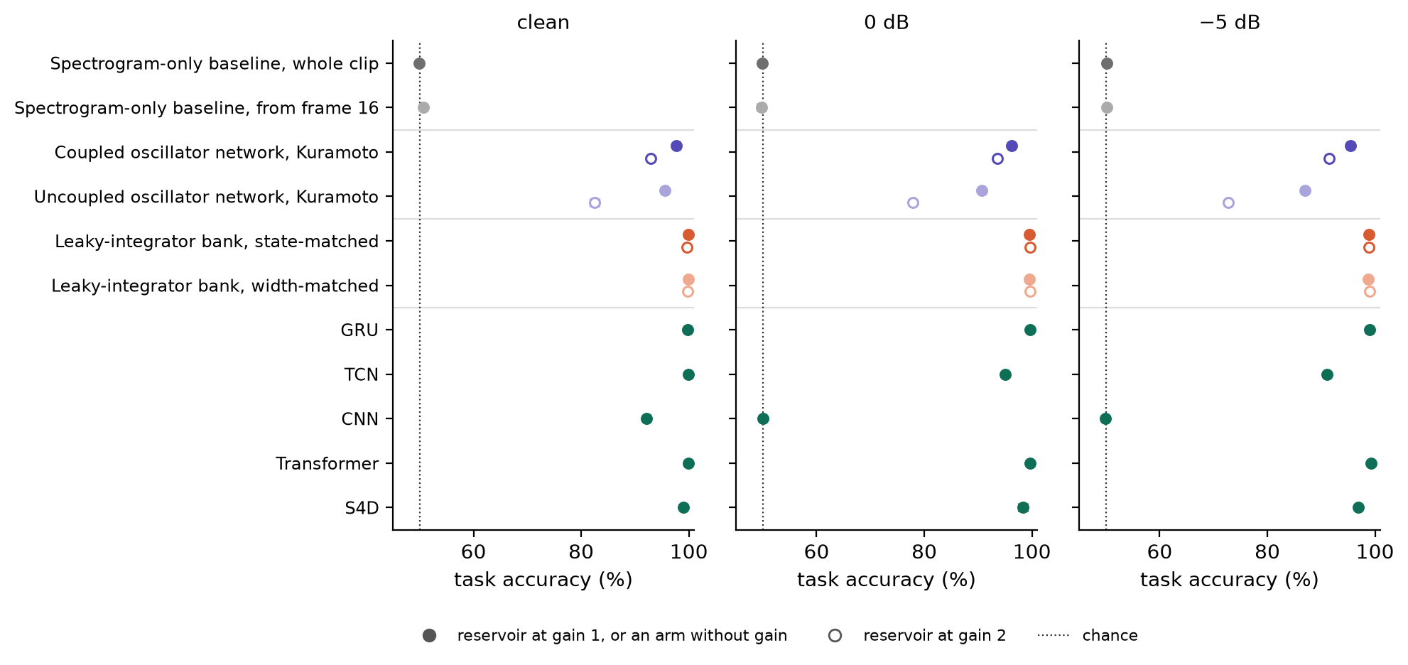
Temporal order. The controls experiment also runs a second task, built so that an order-free read of the input cannot solve it: two digits spoken one after the other, and the question is which came first. The mean and spread of a signal do not depend on the order of its frames, so the spectrogram-only baseline, read over the whole span, sits at 50% by construction. Anything above that has to come from an arm’s memory of what happened when.
Eight experiments
The study runs these comparisons, and the ablations of the next section, as eight experiments.
| experiment | runs | what it asks |
|---|---|---|
| leak check | 13 | Does the pipeline leak? Every reservoir with no input must read exactly chance, and a per-clip read window is measured for how much it would give away. |
| controls | 852 | Does the network add anything beyond its input, a leaky-integrator bank of its size, or its own oscillators uncoupled, and how do trained baselines compare? On recognition and on temporal order. |
| design | 3,744 | Does the network’s design matter: its coupling function, lattice geometry, natural frequencies, restoring strength and coupling ceiling? |
| cochlea | 432 | Do a coil and a cochlea, lattices built to follow the ear, do better than the torus? |
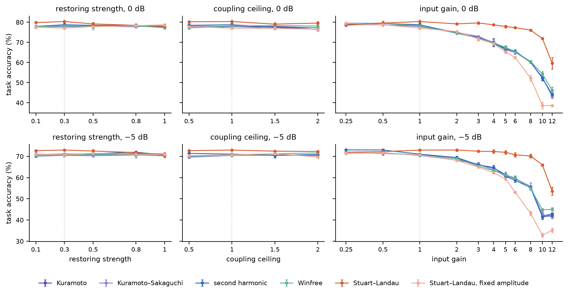
| sweep | 684 | What happens beyond the design’s levels: restoring strengths up to 1, ceilings of 1.5 and 2, and input gains from 0.25 to 12? |
| quadrature | 126 | Can the networks use a drive that tells them when in a band’s cycle to push (section 08)? |
| projection | 432 | Does the readout’s fixed random projection matter? The reservoirs are read again through one drawn from each run’s seed. |
| Becker folds | 70 | Where do the arms sit against published AudioMNIST results, on the corpus’s own speaker folds? |
07 · the ablationsChanging the physics one factor at a time
The design experiment asks whether the design of the network matters. It crosses five factors of the coupled network, 312 configurations at 0 and −5 dB, both gains and three seeds, and measures every effect on matched pairs: two runs identical in every factor but the one compared, at the same noise level, gain and seed.
The coupling function
How the phases of two coupled oscillators turn into a push on one of them. The paper tests six, each a standard object in the synchronization literature, each changing one property of the pull.
| function | the coupling term for oscillator i | what it changes |
|---|---|---|
| Kuramoto | Σ Kij sin(θj − θi) | The reference: each oscillator pulled toward the others’ phases. |
| Kuramoto–Sakaguchi | Σ Kij sin(θj − θi − π/4) | A phase lag that breaks the pull’s symmetry and admits travelling waves. |
| second harmonic | Kuramoto + ½ Σ Kij sin 2(θj − θi) | Favours two-cluster states: pairs in phase or in opposition. |
| Winfree | −sin θi Σ Kij (1 + cos θj) | How strongly an oscillator responds, and acts, depends on its own phase. |
| Stuart–Landau | Σ Kij (zj − zi), z = x + iy | Amplitude joins phase as state: each oscillator relaxes to a cycle of radius 1. |
| Stuart–Landau, fixed amplitude | the same, |z| held at 1 | The phase-only limit, which reduces to Kuramoto: it separates what amplitude adds. |
The lattice geometry
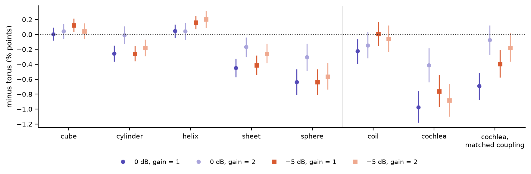
Every geometry stores the same 256 oscillators per channel in the same 16 × 16 grid, with row r driven by band r. A geometry only changes how the grid’s edges are glued, and so which oscillators are neighbours. The kernel is the same table of weights in every case; the gluing decides where each weight lands. The design experiment runs six geometries. The cochlea experiment adds two that follow the ear itself: a coil, the 256 oscillators on one open spiral from the apex (the lowest band) to the base (the highest), an octave per turn, and a cochlea, the coil with two features of the cochlea’s mechanics. Influence runs three times as strongly from base to apex as back, as the travelling wave does, and the coupling into each site grows with the spiral’s curvature, from a quarter at the base to full strength at the apex. Because that weighting halves the cochlea’s average coupling, a control keeps its shape at the coil’s average. Click any oscillator on the grid to see who acts on it.
The other three factors
- Natural frequencies. Random, drawn from N(1, 0.1²); tonotopic, each row set to the centre frequency of the mel band that drives it, with small jitter, the arrangement of the cochlea; identical, all 1.
- Restoring strength λ. 0.3 and 0.1: a longer or shorter memory.
- Coupling ceiling. 1 and 0.5: stronger or weaker coupling overall.
The two Stuart–Landau functions were run on the torus only, a limit of the study’s scope: their core was built for the torus, and the other geometries were wired into the phase oscillators alone. The sweep experiment then pushes each coupling function’s reference network past these levels, to restoring strengths of 0.5 to 1, ceilings of 1.5 and 2, and gains from 0.25 to 12. The console below runs the random-frequency slice of the design and cochlea experiments: every coupling function on every geometry it was run on, at restoring strength 0.3 and coupling ceiling 1.
08 · the drive signalTwo input pathways
Everything so far drives the oscillators with the spectrogram: how loud each band is, frame by frame. That throws away something an oscillator could use. Sound is itself oscillation, and a spectrogram drive tells an oscillator how hard to push, never when in the sound’s own cycle to push. An oscillator nudged at the right moment of every cycle can lock to a rhythm; one pushed at random moments cannot. So the paper also drives the network through a pathway that keeps timing, with its own spectrogram-only baseline.
- Spectrogram. The front end of section 04: each band’s energy adds to the turning rate of its row, the same push whatever the oscillator’s phase. Everything above runs on it.
- Quadrature. Each band’s energy and phase, 62.5 times a second: the phase of the band’s centre frequency, demodulated so what remains is how the band drifts around that centre (within ±31 Hz). The push becomes g · A · sin(φ − θ): it depends on where the oscillator is relative to the band’s own cycle, the phase-referenced drive Adler analysed in 1946, which pulls an oscillator into step with the band.
The paper runs the quadrature pathway on coupled networks only, the four phase coupling functions on the torus: a leaky integrator has no phase for the push to act on, and the question is whether coupled oscillators can use a phase-referenced drive at all. The console below adds the uncoupled network on the quadrature pathway, which the paper did not run, as the obvious reference.
09 · run it yourselfThe experiment, one clip at a time
Everything below runs in your browser: the front end, the model, the read and the readout, with the physics ported line for line from the paper’s harness and the readout for each condition fitted exactly the way the paper fits it. Pick a model, a pathway and a condition, pick a recording or record yourself saying a digit, and press play. The clip is heard and the network is driven at the same moment; the scores appear when the read’s last window closes.
Gain and noise snap to the levels the paper ran (gains 1 and 2; clean, 0 dB and −5 dB). Where the paper did not run a combination you pick, the console moves the other settings to the nearest one it did and says so under the controls. Each prediction comes from a readout fitted at exactly that condition at seed 0, and the accuracy beside it is the paper’s, over all three seeds.
10 · what we foundMostly the input, and a memory
Against its controls. Read at the common width, the spectrogram alone reads 93.6% on clean audio, 78.0% at 0 dB and 71.6% at −5 dB. The Kuramoto network at gain 1 reads 91.1%, 77.8% and 70.7%: within a point of its own input with noise, and 2.5 points below it on clean audio. It reads 0.4 to 1.1 points above the same network uncoupled, and about 4 points above the state-matched leaky-integrator bank with noise, though 2.35 below it on clean audio. With noise every trained baseline reads above it, from 79.2% (CNN) to 82.8% (GRU) at 0 dB.
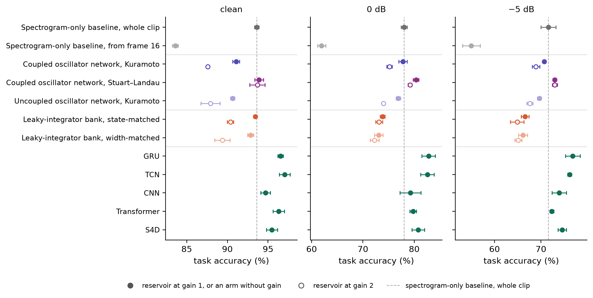
What the dynamics add is memory. Read only after its 16-frame warm-up, the network reads 7.5 to 15.9 points above its input read over the same frames: it carries the onset, which the input loses without its first 16 frames. On the order task, which the input alone cannot solve (49.8% to 50.6%), it reads 95.5% to 97.7%. The leaky-integrator banks do both, and better on order, 98.7% to 99.9%. The reason is the same in both: apart from the restoring pull and the coupling, an oscillator’s phase is the running sum of its band’s energy wrapped around a circle. Oscillation adds no memory the bank lacks; the phase is an integrator whose sum wraps. Coupling adds about a point on noisy recognition and 2 to 19 points on order.
Design. Among phase oscillators, the coupling function moved accuracy by at most half a point, and every lattice geometry read within 0.65 points of the torus. The coil read within 0.22 points of it and the cochlea 0.41 to 0.97 below: built to follow the ear, they read no better. The one design choice that mattered was a free amplitude. The Stuart–Landau network reads 2.1 to 3.8 points above its Kuramoto match and, at the reference configuration, above its own input in every noisy condition, by 1.1 to 2.3 points, which puts it in the trained baselines’ range. With its amplitude fixed it reads like Kuramoto, so the effect is the amplitude, not the coupling form.
Gain and drive. Gain separates the Stuart–Landau network from the rest: from gain 1 to gain 8 it lost 3 to 4 points while every phase-oscillator network lost 15 to 19, as if a free amplitude lets an oscillator absorb a strong drive in its radius where a phase can only be pushed faster. Below gain 1 the order reverses, and at their better low gain the phase networks read above their input at 0 dB. Driven in quadrature, every network read near chance, 11.7% to 15.1%: in no run did more than 0.3% of its oscillators lock to their band.
The readout. Widening the readout to 4,096 features lifts the reservoirs above their input, but through a readout with 21 times as many fitted weights, so the fair comparison stays at the common width. More training data helps the trained baselines three to six times as much as the network, since in a reservoir only the readout learns.
In short. Untrained and read at a common width, a coupled oscillator network classifies noisy, held-out spoken digits about as well as its own input, and carries the order of events by integrating it, as a leaky-integrator bank does. Coupling adds a little to both; a free amplitude lifts it above its input and into the trained baselines’ range; the geometry and the phase coupling function each move it by less than a point. Those numbers are the baseline a trained oscillator network of this size, on this task, should beat.
11 · go deeperThe paper, the code and the prior art
The paper, the harness that ran every model on this page, and the per-run record behind every number quoted here are public. The browser code here is a port of that harness, checked against it: the scores your browser computes match the harness’s on every demo clip, and every untrained arm’s readout, rescored on the full test set, reproduces the paper’s seed-0 accuracy.
Read the paper (PDF) →Its code and record on GitHub →
Further reading
- How a machine hears a number: the first post, from pressure waves to an oscillator core
- oscillator-research: every paper in this programme, with its code and data
- Kuramoto (1975): the minimal model of synchronization
- Sakaguchi and Kuramoto (1986): the phase-lagged coupling
- Winfree (1967): phase response and influence
- Adler (1946): locking an oscillator to an injected signal
- Aranson and Kramer (2002): the complex Ginzburg–Landau equation, Stuart–Landau’s field
- Jaeger (2001) and Maass et al. (2002): reservoir computing
- Jaeger et al. (2007): leaky-integrator echo state networks
- Becker et al. (2024): AudioMNIST, and the speaker folds used for comparison with published results
- Abreu Araujo et al. (2020): how much of an oscillator reservoir’s accuracy its front end supplies
- Kryski (2026): the survey of oscillator networks in machine learning that found these ablations missing