How a machine hears a number.

01 — the problemSound is a terrible input format

Say “seven” out loud. Your vocal folds chop an airflow into pulses, your throat and mouth shape those pulses into resonances, and a pressure wave leaves your face at about 340 m/s. A microphone measures that pressure 16,000 times a second and writes down a number each time. One second of speech is a list of 16,000 numbers.

Pick a digit below and look at what a model is actually handed.

The fix is a hundred years older than deep learning: stop describing the wave and start describing which frequencies are present, and when. Two recordings of “seven” differ enormously sample by sample, and look almost the same once you plot them that way. Everything in the rest of this guide — every architecture, conventional or exotic — sits behind that same transformation.

02 — the fourier transformOne slice, taken apart into pure tones

Fourier’s claim: any wave, however jagged, is a sum of plain sine waves at different frequencies, amplitudes, and phase offsets. The Fast Fourier Transform (FFT) is the algorithm that finds those ingredients — it takes a block of samples and returns, for each frequency, how much of it is in there.

The catch is in the word block. An FFT over a whole second tells you every frequency the second contained, and nothing about the order they arrived in. “Seven” and “teevn” would come out identical. So we take a small block — 512 samples here, 32 milliseconds, short enough that the mouth barely moves — and analyze that.

03 — the STFTSlide the window: a picture of sound

The Short-Time Fourier Transform (STFT) is just the previous figure on repeat: take a window, FFT it, shift the window forward by a fixed hop, repeat to the end of the file, and stack the results side by side. The result is a spectrogram: time along the x-axis, frequency up the y-axis, brightness for energy.

Two parameters set the whole grid, and they trade against each other. A longer window resolves frequency more finely but smears events in time; a shorter one localizes the click of a “t” but cannot tell 300 Hz from 320 Hz. The settings used throughout this guide are the ones the digit experiments actually use: a 512-sample window (n_fft = 512, 32 ms) hopping 256 samples (16 ms), which yields 62.5 frames per second — one frame per 16 ms of speech.

Before the STFT, each window is multiplied by a smooth bell (a Hann window). Cutting a block out with hard edges would add a click the FFT dutifully reports as high-frequency energy that is not in the signal; tapering the edges removes it.

04 — the mel scaleRebuilding the axis around the ear

257 frequency bins, evenly spaced from 0 to 8 kHz, is not how hearing works. The gap between 100 Hz and 200 Hz is obvious to anyone; the gap between 6,000 Hz and 6,100 Hz is inaudible, though both are 100 Hz. Resolution in the ear is roughly logarithmic — fine at the bottom, coarse at the top.

The mel scale (from “melody”) is the warped frequency axis where equal distances sound like equal pitch steps. The common formula is mel = 2595 · log₁₀(1 + Hz / 700), near-linear below 1 kHz and increasingly compressive above it.

Press play below and watch which filters actually fire while the digit is spoken.

One more step, and it matters more than it looks. Loudness is perceived logarithmically too, so we take the log of each band’s energy. That turns the ratios that matter into differences a network can add and subtract, and it stops one loud vowel from dominating the numbers. STFT → mel filterbank → log is the standard audio front end; the result is the log-mel spectrogram.

05 — the standard stackAn encoder, and three ways out

With the front end fixed, the rest of a speech system has a common shape: an encoder that turns the mel frames into a sequence of learned feature vectors, and a decoder that converts those into whatever you want out. Almost every well-known model is a choice of encoder (CNN, RNN/LSTM, Conformer, Transformer, state-space model) crossed with a choice of decoder.

What the training data has to be

Getting back out to audio: the phase problem

Classification and transcription end at a small output. Generating audio does not, and it runs into a wall that is worth understanding, because it explains why half the field exists.

The STFT produces complex numbers: a magnitude (how much of this frequency) and a phase (where in its cycle that frequency is at this instant). A spectrogram displays magnitude only; the mel filterbank then throws away even the fine frequency detail. The inverse STFT (iSTFT) — inverse FFT per frame, then overlap-add the frames back together — reconstructs the waveform perfectly, but only if you give it both parts. Hand it magnitudes with no phase and the overlapping frames fight each other instead of adding up, and you get a smeared, metallic buzz.

So a generative audio model must supply the missing phase. Three eras of answers:

• Griffin–Lim (algorithmic). Guess a phase, iSTFT, re-STFT, keep the target magnitudes and the newly implied phase, repeat. Converges to something playable and famously robotic. Where you have heard it: the original Tacotron (2017) shipped with Griffin–Lim, which is exactly why first-generation neural TTS demos had that ringing, underwater timbre — and why librosa’s griffinlim is still the two-line baseline everyone tries first.
• Neural vocoders (the modern default). A network trained on thousands of hours of real speech maps mel frames straight to samples. It never “solves” for phase; it has learned what real glottal pulses, real fricative noise, and real micro-jitter look like. Where you have heard them: WaveNet (2016) predicted one sample at a time — stunning, and far too slow, so Tacotron 2 paired it with a mel decoder; HiFi-GAN (2020) made GAN vocoding fast and clean enough to become the default, and it is the vocoder inside Kokoro and StyleTTS 2; BigVGAN scaled it to universal, any-voice audio; DiffWave and WaveGrad sculpt noise into a waveform by diffusion; and Vocos predicts STFT coefficients — magnitude and phase — then lets a single iSTFT do the synthesis, which is fast enough to be the interesting compromise.
• Multi-resolution spectral losses. Whatever the generator, training compares the output to the target through several STFTs at once — short windows to police clicks and transients, long windows to police pitch and vowels. Where it comes from: Parallel WaveGAN (2019) introduced the multi-resolution STFT loss that nearly every vocoder since has adopted, including HiFi-GAN’s mel loss and SoundStream/EnCodec’s spectral reconstruction terms; the differentiable-DSP line (DDSP) leans on the same idea.

Text-to-speech is not simply speech-to-text backwards

Structurally it mirrors: text encoder → acoustic decoder → vocoder → wave. In difficulty it does not. Recognition is many-to-one: a thousand different performances of “seven” must collapse onto one string, so the model’s job is to throw variation away. Synthesis is one-to-many: from five letters the model must invent a speaker, a pitch contour, a speaking rate, the emphasis, and the breaths. Nothing in the input says which of the infinitely many correct readings to produce, which is why modern TTS spends its parameters on duration predictors, style/speaker embeddings, and generative decoders.

06 — a different coreWhat if the middle box were physics?

Everything above treats the encoder as a stack of matrix multiplications. Here is the alternative Project Resonant is built to test: replace it with a population of coupled oscillators, and let the audio drive them.

The motivation is not aesthetic. Speech is oscillation — vocal folds cycling, resonances ringing, syllables at 4–8 Hz. A representation whose internal state is also a set of phases and frequencies starts closer to its data than a general-purpose matrix stack does. And the entire history of the signal lives in a fixed-size state — the phases — instead of a context window that grows with time.

The stadium crowd

Imagine a stadium at a concert, everyone holding their phone with the light on, each person swinging it in a slow windmill while their favourite singer plays.

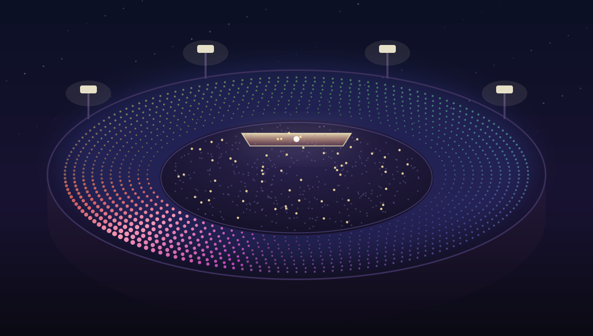
• Where each person’s light is pointing right now is that oscillator’s phase, θ. It swings around and around; straight up at 0 and at 2π is the same place in the circle.
• Everyone has a preferred swing tempo, ω — the speed they would settle into if nobody else were there.
• People glance at their neighbours and adjust: the coupling. You speed up or slow down depending on whether the lights beside you are ahead of yours or behind it.
• The music from the stage pushes the whole section on the beat: the drive. This is where the audio enters — a loud low note leans on one part of the crowd, a bright cymbal on another.
• A gentle tendency to let your arm drop keeps the whole thing from running away: the pinning.
• The seating chart never changes. Nobody swaps seats — only the wave of light moves through them.

Written down, that is the Kuramoto model, one of the most studied equations in physics — it is how fireflies end up flashing together and how metronomes on a shared board come into step. Each oscillator updates its phase like this:

Coupling strength is the interesting dial. Too weak and every oscillator ignores the others — a bag of independent filters. Too strong and the entire population locks into one rigid clump that reports nothing except “loud”. The useful regime is in between, where parts of the field synchronize and parts do not, and which parts depends on what it is hearing.

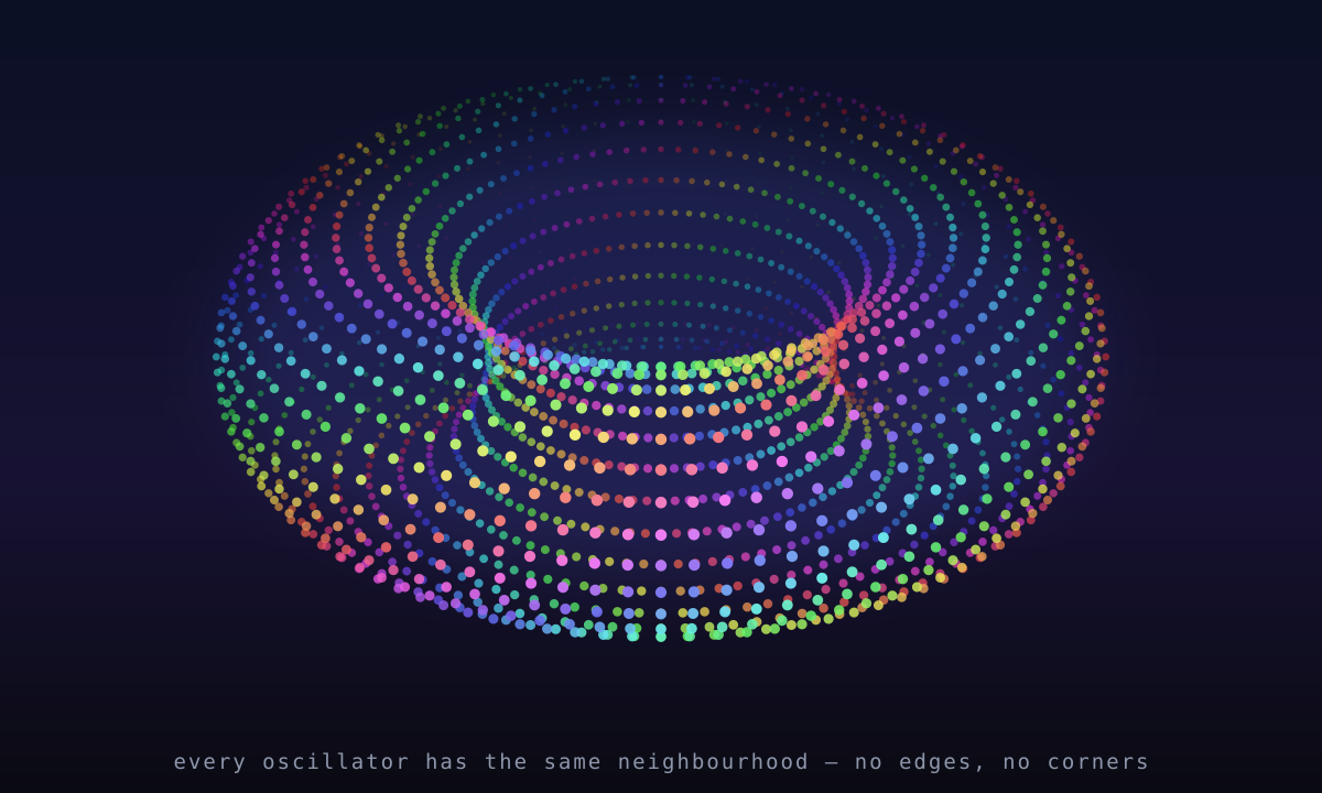
Why a torus

The oscillators are not a loose bag; they sit on a 16 × 16 grid, and coupling depends only on the offset between two cells, not their absolute position — the same neighbourhood rule everywhere, which is exactly what makes a convolution a convolution. Rows are frequency bands (mel band b drives grid row b, so the grid inherits the ear’s layout); columns are a second dimension the dynamics can spread into.

Both axes wrap: the last row’s neighbour is the first row, the last column’s neighbour is the first column. A grid with both edges glued is a torus. Two reasons it is worth the trouble. First, no edges means no special cases — every oscillator has an identical neighbourhood, so one small kernel describes the whole field. Second, a translation-invariant kernel on a periodic grid is a circular convolution, which is a pointwise multiply in Fourier space: coupling all 256 oscillators to all 256 others costs one FFT rather than a 256 × 256 matrix. The physics of the configuration on this page is about 2,000 numbers.

Reading a physical system

You cannot feed phases to a classifier directly — θ = 0.01 and θ = 6.27 are neighbours on the circle but look far apart as numbers. So the readout takes sin θ and cos θ, which are smooth around the wrap, and summarizes each oscillator over the clip with four numbers: mean sin and mean cos (where it sat) and the mean sin and cos of its per-frame phase step (how fast it turned — an oscillator captured by the stimulus reports the stimulus’s rhythm, a free one reports its own). With 4 channels × 256 cells that is 4,096 features, and a plain linear layer on top.

07 — watch it runThe whole pipeline, live

Below, everything on this page runs end to end. Pick a digit and press play: the clip is analyzed into mel bands, the bands are injected into the oscillator field, 61 frames of physics are integrated, and the linear readout reports what it thinks it heard — all in your browser, in about the time it takes to blink. Or press record and say a digit yourself, and your own voice goes through the same path.

One thing to be clear about before you look: the physics here is not trained. The coupling kernel is a random draw that was never touched by gradient descent, the natural frequencies were designed by hand, and the only fitted part is the final linear layer. On held-out speakers this configuration gets — of ten-way digits right. That is a statement about how much structure raw oscillator dynamics impose on their input — and section 08 runs the control that says how much of it the coupling deserves credit for. It is not a claim that any of this beats a trained network.

08 — this is just the beginningWhat this shows, and what it doesn’t

Spoken digits are an easy task with a long history — they are the “hello world” of speech, and a physical spin-torque oscillator hit 99.6% on a comparable benchmark back in 2017. A high number here is not evidence that oscillator cores beat transformers at speech. What the demo does show, concretely:

• Untrained dynamics carry usable structure. No gradient touched the kernel. The audio drives the field, the field organizes, and a linear probe reads the digit off the result.
• The state is fixed-size and streaming. 4 × 256 phases at every frame, whatever the length of the input. No cache grows.
• The whole model is tiny. The physics is roughly 2,000 numbers, and it simulates a second of audio in a browser tab in a few dozen milliseconds.

How much of it is the synchronization?

There are two different machines hiding in that description, and it is worth separating them. One is a bank of independent resonators: 1,024 oscillators, each tuned to a frequency band, each shoved by its own slice of the audio, none of them aware of any other. That is a perfectly good feature extractor, and it is not a new idea — it is what a filterbank does. The other is the coupled field: the same oscillators, now allowed to pull on their neighbours, so what any one of them does depends on what the ones around it are doing. Only the second one is a synchronization model.

The difference between them is a single number — the coupling kernel. Set it to zero and the neighbours stop listening to each other; everything else stays identical. Fit the same linear readout on each and you can price the coupling directly:

Two points. On spoken digits, letting the oscillators talk to each other is worth about two points over letting them ring independently — real, repeatable across seeds, and much smaller than the headline number would suggest. Most of the work is being done by the resonator bank and a generous linear readout.

The third row is a different kind of statement, and it is the one most likely to be misread. It is not a measurement of the coupling; it is what happens when you change the machine and keep the old readout. The linear layer was fitted to one physical system and handed a different one, so it fails — the way a key fails in a lock it was not cut for. The physics is fine. The translation is stale.

Why does a two-point gap still matter? Because of what is being compared. A resonator bank is a fixed function: each oscillator's response is decided the moment you choose its frequency. A coupled field has a shape that can be changed — the kernel says who listens to whom and how strongly, and that shape is what makes patterns like travelling waves and partial synchronization possible at all. Here that shape is a random draw that no gradient ever touched, and it still buys two points. The interesting question is not whether an arbitrary coupling helps a little; it is what a good one does.

There are two obvious ways to find out, and both are open. Train it: the kernel is a small, differentiable parameter set, so gradient descent can shape who couples to whom instead of leaving it to chance. Change the physics: Kuramoto's sin(θⱼ − θᵢ) is only the simplest way for two oscillators to interact. Add a phase lag and you get travelling waves; add a second harmonic and the population splits into clusters instead of one clump; amplitude-carrying oscillators can express loudness as well as timing. Each is a different coupling law over the same field, and each is being worked through with the same discipline as everything else here — a parameter-matched control and a bar written down first.

Where this goes

The open question is whether the wave-physics prior is a genuinely better architecture for wave-shaped input and output — real-time speech in and out of one interruptible, context-carrying core — or whether it is a beautiful idea that a boring stack of matrices beats at every size. The repository is built so that the hypothesis can fail cleanly: parameter-matched controls, frozen baselines, immutable training logs, and verdicts written before the runs. That work is ongoing, and the interesting part is still ahead.

09 — go deeperThe code, and the prior art

Everything on this page — the front end, the oscillator core, the readout, and the ten recordings — comes out of a research repository that holds the hypothesis, the architecture, every experiment log, and the results that refuted my own expectations. It is getting a clean-up pass before it goes public; the link will land here when it does.

Prior art worth reading